4 januari 2014

Simulate wet surface with screen space reflection

A wet surface will reflect some of the light, but reflections are computationally expensive. Using a deferred shader, it is possible to simulate this reflection (fresnel reflection) to the second stage. The basic idea is simple: If a pixel should reflect, a ray tracing algorithm is used to compute where the reflected ray will hit the background.

We don't want to trace the ray through the real geometry, which would be expensive. Instead, it is computed what pixel it corresponds to from the G-buffer of the deferred shader. The data we need from the defered shader is: World position, normals and colors.

To do the actual ray tracing, an iterative algorithm is needed. The reflected vector is first computed, and then incrementally added to the world position of the point we start with. This is repeated as long as needed.

There are a couple of problems that limit the use of this technology:
  1. The reflected ray can point backward to the camera and hit the near cutting plane of the view frustum.
  2. The reflected ray can point sideways, and go outside of the screen.
  3. The reflected ray can hit a pixel that is hidden behind a near object.
  4. The increment used in the algorithm should be small to get a good resolution of the eventual target point, which will force the use of many iterations and high evaluation costs.
These all sound like severe limitations, but it turns out that wet surface reflection can still be done effectively:
  1. The Fresnel reflection has the effect of reflecting most for incoming light at large angles to the normal. That means that light reflecting backward toward the camera can be ignored.
  2. Wet surfaces are typically rough. This can be simulated with some random noise, which can hide the effect where some ray reflections couldn't be determined.
  3. The iteration can start out with a small delta, and increase it exponentially. That way, it can be possible to get good resolution on short distances, while still being possible to compute long distances.
The following is an example fragment shader to help calibrate the constants:

// Create a float value 0 to 1 into a color from red, through green and then blue.
vec4 rainbow(float x) {
	float level = x * 2.0;
	float r, g, b;
	if (level <= 0) {
		r = g = b = 0;
	} else if (level <= 1) {
		r = mix(1, 0, level);
		g = mix(0, 1, level);
		b = 0;
	} else if (level > 1) {
		r = 0;
		g = mix(1, 0, level-1);
		b = mix(0, 1, level-1);
	}
	return vec4(r, g, b, 1);
}

uniform sampler2D colTex;     // Color texture sampler
uniform sampler2D posTex;     // World position texture sampler
uniform sampler2D normalTex;  // Normal texture sampler
in vec2 screen;               // The screen position (0 to 1)

layout(location = 0) out vec4 color;

void main(void)
{
	vec3 worldStartingPos = texture(posTex, screen).xyz;
	vec3 normal = texture(normalTex, screen).xyz;
	vec3 cameraToWorld = worldStartingPos.xyz - UBOCamera.xyz;
	float cameraToWorldDist = length(cameraToWorld);
	vec3 cameraToWorldNorm = normalize(cameraToWorld);
	vec3 refl = normalize(reflect(cameraToWorldNorm, normal)); // This is the reflection vector

	if (dot(refl, cameraToWorldNorm) < 0) {
		// Ignore reflections going backwards towards the camera, indicate with white
		color = vec4(1,1,1,1);
		return;
	}

	vec3 newPos;
	vec4 newScreen;
	float i = 0;
	vec3 rayTrace = worldStartingPos;
	float currentWorldDist, rayDist;
	float incr = 0.4;
	do {
		i += 0.05;
		rayTrace += refl*incr;
		incr *= 1.3;
		newScreen = UBOProjectionviewMatrix * vec4(rayTrace, 1);
		newScreen /= newScreen.w;
		newPos = texture(posTex, newScreen.xy/2.0+0.5).xyz;
		currentWorldDist = length(newPos.xyz - UBOCamera.xyz);
		rayDist = length(rayTrace.xyz - UBOCamera.xyz);
		if (newScreen.x > 1 || newScreen.x < -1 || newScreen.y > 1 || newScreen.y < -1 || newScreen.z > 1 || newScreen.z < -1 || i >= 1.0 || cameraToWorldDist > currentWorldDist) {
			break; // This is a failure mode.
		}
	} while(rayDist < currentWorldDist);

	if (cameraToWorldDist > currentWorldDist)
		color = vec4(1,1,0,1); // Yellow indicates we found a pixel hidden behind another object
	else if (newScreen.x > 1 || newScreen.x < -1 || newScreen.y > 1 || newScreen.y < -1)
		color = vec4(0,0,0,1); // Black used for outside of screen
	else if (newScreen.z > 1 && newScreen.z < -1)
		color = vec4(1,1,1,1); // White outside of frustum
	else
		color = rainbow(i); // Encode number of iterations as a color. Red, then green and last blue
	return;
}
The shader doesn't implement the actual reflection, but will show color coded information. White is used to indicate a reflection going back to the camera, yellow indicates a pixel hidden behind another object, black indicates we got outside of the screen. Finally, a rainbow code is used to indicate the number of iterations needed to find the target. Red is 1, then green and finally blue for maximum.

The example code will do at max 20 iterations (increment i with 0.05). Notice how the delta gradually is increased (incr is increased by 30% every iteration at line 50). Starting with a color texture as follows:
Original
And then applying the shader above, the result is:

Calibration mode
Please ignore the red and yellow sky, and look at the big block in the foreground. Much of it is white, because that reflects mostly back to the camera. The left side, however, has several colors. Black indicates a ray that goes outside of the picture, but the spectrum from red to blue indicates successful ray tracing. The bottom is red, which is logical as the reflection will immediately hit the near ground. The trees are found at median distance, indicated by green. And the sky is blue, which means a maximum number of iterations was needed to hit the sky pixel.

Notice that the single monster is reflected twice, at two different iterations. This is an effect of iterating in big steps.

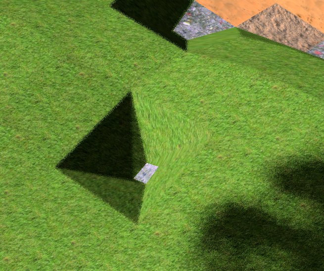
Next is a picture from inside a cave, with no reflections enabled:
Caves without reflections
The same view, but with reflections enabled:
Caves with reflections
In this picture, the normals were manipulated randomly, and the original pixel color is blended with the reflected color depending on the angle. The final fragment shader source code for this is:

// Create a float value 0 to 1 into a color from red, through green and then blue.
vec4 rainbow(float x) {
	float level = x * 2.0;
	float r, g, b;
	if (level <= 0) {
		r = g = b = 0;
	} else if (level <= 1) {
		r = mix(1, 0, level);
		g = mix(0, 1, level);
		b = 0;
	} else if (level > 1) {
		r = 0;
		g = mix(1, 0, level-1);
		b = mix(0, 1, level-1);
	}
	return vec4(r, g, b, 1);
}

// Return a random value between -1 and +1.
float noise(vec3 v) {
	return snoise((v.xy+v.z)*10);
}

uniform sampler2D colTex;     // Color texture sampler
uniform sampler2D posTex;     // World position texture sampler
uniform sampler2D normalTex;  // Normal texture sampler
uniform usampler2D materialTex;  // Material texture sampler
in vec2 screen;               // The screen position (0 to 1)

layout(location = 0) out vec4 color;

// #define CALIBRATE // Define this to get a color coded representation of number of needed iterations
void main(void)
{
	vec4 origColor = texture(colTex, screen);
	uint effectType = texture(materialTex, screen).r & 0xf; // High nibbles are used for modulating factor
	if (effectType != 1) {
		color = origColor;
		return;
	}
	vec3 worldStartingPos = texture(posTex, screen).xyz;
	vec3 normal = texture(normalTex, screen).xyz;
	vec3 cameraToWorld = worldStartingPos.xyz - UBOCamera.xyz;
	float cameraToWorldDist = length(cameraToWorld);
	float scaleNormal = max(3.0, cameraToWorldDist*1.5);
#ifndef CALIBRATE
	normal.x += noise(worldStartingPos)/scaleNormal;
	normal.y += noise(worldStartingPos+100)/scaleNormal;
#endif
	vec3 cameraToWorldNorm = normalize(cameraToWorld);
	vec3 refl = normalize(reflect(cameraToWorldNorm, normal)); // This is the reflection vector
#ifdef CALIBRATE
	if (dot(refl, cameraToWorldNorm) < 0) {
		// Ignore reflections going backwards towards the camera, indicate with white
		color = vec4(1,1,1,1);
		return;
	}
#endif
	float cosAngle = abs(dot(normal, cameraToWorldNorm)); // Will be a value between 0 and 1
	float fact = 1 - cosAngle;
	fact = min(1, 1.38 - fact*fact);
#ifndef CALIBRATE
	if (fact > 0.95) {
		color = origColor;
		return;
	}
#endif // CALIBRATE
	vec3 newPos;
	vec4 newScreen;
	float i = 0;
	vec3 rayTrace = worldStartingPos;
	float currentWorldDist, rayDist;
	float incr = 0.4;
	do {
		i += 0.05;
		rayTrace += refl*incr;
		incr *= 1.3;
		newScreen = UBOProjectionviewMatrix * vec4(rayTrace, 1);
		newScreen /= newScreen.w;
		newPos = texture(posTex, newScreen.xy/2.0+0.5).xyz;
		currentWorldDist = length(newPos.xyz - UBOCamera.xyz);
		rayDist = length(rayTrace.xyz - UBOCamera.xyz);
		if (newScreen.x > 1 || newScreen.x < -1 || newScreen.y > 1 || newScreen.y < -1 || newScreen.z > 1 || newScreen.z < -1 || i >= 1.0 || cameraToWorldDist > currentWorldDist) {
			fact = 1.0; // Ignore any reflection
			break; // This is a failure mode.
		}
	} while(rayDist < currentWorldDist);
	// } while(0);
#ifdef CALIBRATE
	if (cameraToWorldDist > currentWorldDist)
		color = vec4(1,1,0,1); // Yellow indicates we found a pixel hidden behind another object
	else if (newScreen.x > 1 || newScreen.x < -1 || newScreen.y > 1 || newScreen.y < -1)
		color = vec4(0,0,0,1); // Black used for outside of screen
	else if (newScreen.z > 1 && newScreen.z < -1)
		color = vec4(1,1,1,1); // White outside of frustum
	else
		color = rainbow(i); // Encode number of iterations as a color. Red, then green, and last blue.
	return;
#endif
	vec4 newColor = texture(colTex, newScreen.xy/2.0 + 0.5);
	if (dot(refl, cameraToWorldNorm) < 0)
		fact = 1.0; // Ignore reflections going backwards towards the camera
	else if (newScreen.x > 1 || newScreen.x < -1 || newScreen.y > 1 || newScreen.y < -1)
		fact = 1.0; // Falling outside of screen
	else if (cameraToWorldDist > currentWorldDist)
		fact = 1.0;
	color = origColor*fact + newColor*(1-fact);
}

The source code for this can be found at the Ephenation ScreenSpaceReflection.glsl. The snoise function is a 2D simplex noise that can be found at Ephenation common.glsl.

22 februari 2013

Ephenation evaluation report

Vision of Ephenation

To have a game like World Of Warcraft, where players are able to add their own adventures. I think this is a probable future development. This type of games should be fully realized and generally available in something like 10 to 20 years.

Goals

Unlimited world

The size of the world should not be limited. It is easier to implement a flat world than a spherical world, and a flat world can be unlimited. The nature will obviously have to be created automatically.

Unlimited players

This is not possible, of course, but the number of simultaneous players should be big. Limitation to 10 or 100 is much too small, as everyone would more or less know everyone and work on the same project. A minimum would be 1000 players, but preferably more than 10000. That will lead into a situation where you always meet new players you don't know, and the world is big enough so as to always find somewhere that you have not explored.

Unlimited levels

Most RPG type of games have a limited set of levels. But that will put a limit on the game play. After reaching the top level, the game is no longer the same. Not only that, but there is a kind of a race to reach this top level. Instead, there shall be no last top level. That will put an emphasis on constant exploration and progress.

Allocate territory

Players should be able to allocate a territory, where they can design their own adventures. This territory shall be protected from others, making sure no one else can interfere with the design.

Social support

The community and social interaction is very important. That is one reason for the requirement to support many players, as it will allow you to include all friends. There are a couple of ways to encourage community:
  1. Use of guilds. This would be a larger group of players, where you know the others.
  2. Temporary teams, used when exploring. It is more fun to explore with others.
  3. Use of common territories. It shall be possible to cooperate with friends to make territories that are related and possibly adjacent to each other.

Mechanics

It shall be possible to design interesting buildings, landscapes and adventures. The adventures shall be advanced enough so as to support triggered actions, with dynamic behavior that depends on player choices.

Execution

This is a description on how the project was executed. It was started end of 2010. Most of the programming was done by me (Lars Pensjö), but I got support with several sub modules.

Server

It was decided to use Go as the programming language for the server. Go has just the right support for this type of software:
  1. High performance (compiled language)
  2. Object oriented and static typing
  3. A concept of gorutines (light version of threads)
  4. A very high quotient for "it works when it compiles"
  5. Garbage collection
The disadvantage of Go when the Ephenation project was started, was that Go was a new language, in transition, with uncertain future. This turned out to not be a problem, and the language has today a frozen specification (Go 1).

To be able to manage the massive amount of players, quadtrees are used for both players and monsters.

It is the server that has full control over all Model data. Player attributes, melee mechanisms, movements, etc.

Client

The client was initially designed in C, but I soon switched to C++. There are still some remains from C, which explains some not-so-good OO solutions. OpenGL was selected, instead of DirectX, partly as a random choice, but also because I wanted to do the development in Linux.

It was decided to use OpenGL 3.3, instead of supporting older variants. There are some nice improvements in OpenGL that makes design easier, which was deemed more important than supporting old hardware.

The world consists of blocks, voxels. This is difficult to draw in real time with high FPS, as the number of faces grow very quickly with viewing distance. Considerable effort was spent on transforming the list of cubes into a list of visible triangles. It is also difficult to make a level of detail (LOD) algorithm that gradually reduce details on long distances.

Another technical difficult with a world based on cubes was to make it look nice, instead of blocky. Some algorithms were investigated that used a kind of filter. As the view distance is limited, there can be a conflict when being underground.

The game engine can't know whether the far distance, which is not visible, should be replaced by a light background (from the sky) or from a dark background (typical to being underground). A compromise is used, where the color of the distance fog depends on the player being at a certain height.

Protocol

There are strict requirements on the protocol. If a server shall be able to handle 10000+ players, the communication can easily become a bottleneck. TCP/IP was selected in favor of UDP/IP, to make it easier to handle traffic control. The protocol itself is not based on any standard, and completely customized for Ephenation.

Mechanics

There are two major choices. Either use a scripting language to control the aspects of the world, or a graphical approach. A scripting language is more powerful, but on the other hand it is harder to learn. There is also the problem with supporting a massive amount of players, in which case time consuming scripts would make it unfeasible.

The choice was to go for a limited set of blocks, with a special block type that can be used to initiate predefined actions. Inspiration was taken from the principles of Lego blocks. With a relatively small set of basic blocks, it is possible to construct the most amazing things.

Evaluation

Game engine

The client side was designed from scratch, instead of using an existing game engine. This may have been a mistake, as the main development time was spent on graphical technology, instead of exploring the basic visions.

Adventure design and mechanics

The set of blocks and possible actions with "activator blocks" are currently limited. It is not enough to construct full adventures that are fun to explore and provides great entertainment.
Early version of the game, where a player abused the monster spawner

Game play

The basic world is automatically generated. This usually make a game of limited interest, as game play is bound to become repetitive. Support from initial players enabled the creation of a world with many new buildings and creations. The more advanced features that support dynamic behavior was not added until later, which unfortunately lead to most part of the current world being too static.

Graphics

The graphics is working, but far from a production level. There are several glitches, e.g. camera falling inside the wall and lighting effects cut off. As the world is dynamic, the possibility to do offline precalculations are limited. That means most graphical effects has to be done live, which is a difficult requirement. For example, it is not known how many light sources that should be possible to manage. It was chosen to use a deferred shader, which improves the decoupling from geometry and shading.
Early attempt to create automatic monsters. This was later replaced with fully animated models.

Social

The social side of the game play has been explored very limited. There are ways to send message to nearby players, and to communicate privately with any player. Although this is a very important aspect of the final vision, it is known technology and not difficult to implement.

Performance tests

The aggressive requirement to support 10,000 simultaneous players is hard to verify. A simple simulator was used, adding 1000 players at random position with a uniform density. These players simply walked around. If they were attacked, they attacked back again. If they were killed, they automatically used the command to revive again.

On a Core I7 with 8 GBytes of RAM, the load from the server was approximately 10%. This is no proof that the server can actually manage 10,000 players, as there may be non linear dependencies. There are known bottlenecks, for example monster management that is currently handled by a single thread. That means at most one core can be used for this, but it should be possible to distribute this task into several smaller goroutines.

The communication was measured at around 100 MB/s. With linear scaling, it would be 1GB/s for 10,000 players. The intention is that the scaling should be linear, as cross communication between players is designed to be of constant volume. Still, it remains to be proven.

There is the obvious question whether the simulator is representative to real players. One way to improve that assessment would be to measure the actual behaviour of real players, and compare with the simulator.

Another possible bottle neck is the communication with the player database (MongoDB). This depends on the number of login/logout and auto saves. It also depends on load generated from the web page. This has not been evaluated. Typically, an access takes about 1ms. The MongoDB is currently located on the same system as the game server, minimizing communication latency. The database will have to be managed by another computer system for a full production server.

Equipment

The objects that the player can wear and wield are simplified. As the game as a concept is unlimited, it is not possible to hand craft objects. Instead, there are 4 defined qualities for each object, per level.

Communication

TCP/IP has a higher overhead than UDP/IP. Some packages are big (the complete chunks), which would have required several UDP/IP packets and a complicated transmission control. It may be that UDP/IP should be used instead. However, this was not an issue for evaluation of the project.

As the server is responsible for all object atributes, the clients need to be updated frequently. Player and monster positions are updated 10 times per second. This generates some data, so the update is limited to nearby players. Because of this, the client need to do interpolation to be able to show smooth movements, and the client need to be able to manage stale information about other players and monsters. The advantage of having the server manage all attributes is that it is not possible to cheat. The client source code is available, and it would have been easy to do changes.

Conclusion

Moore's law

I believe the computers will continue to grow more powerful exponentially for many years still. However, the full power will probably not be accessible unless the game server can scale well with increasing number of cores. The performance test were done on hardware from 2011, and there are already much more powerful equipment available.

Adventure design

As a proof of concept, I think the project was successful. The thing I miss most, is a powerful enough mechanism that supports custom adventures. This is a key point of the game concept, but I believe, with more personnel involved, that new ideas would be available that would improve the possibilities considerably.

Document update history

2013-02-22 First published.
2013-02-24 Added discussion about using voxels on the client side.
2013-02-27 Information about entity attribute management and communication.
2015-05-04 Pictures failed, and were replaced.

5 november 2012

Smooth world from block data


Ephenation is a voxel based world. Everything (almost) are blocks that have a given address. Graphics based on square blocks doesn't look very good. There are ways to make it look good, e.g. the Marching Cubes algorithm.
However, this algorithm has some drawbacks. Every created triangle has a texture, and it is not trivial to decide what texture to use for triangles that span from one block type to another. Another problem is that some cubes in the world shall still be shown as cubes. This leads to difficulties in the transition between smooth terrain and cubistic blocks.

Use of a filter

In Ephenation, it was decided to use another algorithm, with similarities to a low pass filter. The basic idea is to take every coordinate and add a specific delta to each of the three dimensions. The magnitude of the delta is determined as a function of neighbor blocks. A two dimensional example of this could be:
Delta in X dimension
Next, if the same delta is applied in 'y', we get:
Delta in Y dimension
The principle is simple; the delta is computed in every dimension and can be applied independently.

Three dimensions

When computing the delta for 3 dimensions, neighbor vertices has to be take into account from 3 dimensions.

In the figure, there are 8 cubes. They are initially uniformly distributed. The content of these 8 cubes are used to determine the delta of the point P, in the middle, for each of the X, Y and Z dimensions. Only one filter is defined for one dimension, and then the transformation is rotated in three different directions. The algorithm uses a small matrix, of the size 2x2x2, that is initialized with the content of the 8 cubes. The delta computation uses that matrix to determine the delta in one dimension. And then this small matrix is filled with the same content, but rotated for the other dimensions, and the test is repeated.

Merging normals

After applying the delta, it is possible to change the appearance without changing the geometry. If the normals for all triangles that meet at the same vertex is replaced by an average, then it will further increase the smoothness look of the world. To speed up this process, the vertex data is sorted on vertex position. A std::multiset is used, with pointers to the vertex data. This set of pointers is then sorted. A question is whether normals from different materials shall also be averaged. This is not done currently.

There are some special cases that need to be taken care of. For example, it may be that the sum of the normals is a null vector. When that happens, the normals are simply left unchanged.
Non modified normals
And with normals merged, the same geometry will be:
Merged normals

Calibration

The amount of the delta has to be calibrated. See below a video clip where the delta goes from 0 to 0.17.


There is a middle point where the slope is 45 degrees, which corresponds to a calibration constant of 0.125. There is no smooth transition between bitmaps of different kinds. It can be seen in this video clip as a checker pattern. To get smooth transition between different textures is outside of the scope here, and it is not currently implemented in Ephenation.

Texture mapping

Texture UV mapping in a tiled world is trivial. For example, the front face of a cube can be mapped as shown in the picture.
Default UV mapping

When a smoothing filter is applied (coordinates are modified with a delta), it would seem trivial to compute a new UV-mapping. If the new height is decreased from 1 to 0.8 and the lower left is raised by 0.2, then the upper left corner would now be mapped to 0,0.8 instead.
Delta applied on left side
However, there may also be delta added to the Z component. Different deltas can be added to the top and bottom. For the left border in the figure above, the height would still be 0.6 units, but the total length of the left border may be longer as it is could be leaning forward in Z. There are extreme cases, where the total height is approaching 0, but the difference in Z for the left side corners are growing dominant. If only X and Y are used for UV mapping, then the bitmap will appear stretched. This has not been taken care of yet.
The red material is stretched

Chunk borders

In Ephenation, all blocks are organized into chunks. A chunk consists of 32x32x32 blocks organized in a matrix. With a given chunk, it is easy to find individual blocks, as well as adjacent blocks.. But when analyzing blocks at the chunk border, data have to be fetched from another chunk. To simplify this process, the list of neighbor chunks are first prepared. This part of the algorithm is not complete yet, and the border between chunks can be seen as having no delta applied.

Random noise

There is yet another way to improve the realism, and that is to add a random value to the delta. 2D simplex noise is used to add a random noise to the height. The drawback with 2D noise that do not use the height component, is that it will generate the same height delta for all coordinates with the same horizontal coordinates. But that is an acceptable simplification, as it won't be noticeable unless floors above each other are compared. The drawback with 3D simplex noise is that it is more costly.

Special care has to be taken for some materials, like water. It would not look natural to have permanent slopes and hills in the water.

Performance

All together, it is quite a lot of computation that is done to every chunk. With a long viewing distance, a lot of chunks are needed. A thread pool is used for this, using available cores on the CPU. Still, with a 1 or 2 core CPU, the cost can be too high.


Update history

2012-11-11 Use video clip from YouTube instead, to get higher resolution.

26 oktober 2012

Deferred shader part 2

This is a description how deferred shading is used in Ephenation. The algorithm has been separated into a number of stages, that each will update one or more data buffers. The stages and the buffers used for these stages are explained below. Most of the links refer to the actual source code.

Overview

Green box: Shader execution
Blue box: Data stored in a bitmap (of varying formats)
Solid arrow: Indicates data is used
Wide orange arrow: Data is updated

Buffers

There is a depth, diffuse, normal and position buffer allocated. These are common in many deferred shaders, usually called a G buffer, which is described in more detail in part 1.

Light buffer

All lighting effects are added up in a separate channel of type R16F. It is a bitmap texture allocated as follows:
glTexImage2D(GL_TEXTURE_2D, 0, GL_R16F, w, h, 0, G_RED, 0);  
The advantage of having only one channel is that less memory is needed. The disadvantage is that light contributions can not have separate effects for the different colors. The values will typically range from 0 to 1, but can exceed 1 if there are more than one light source (e.g. sun and lamp). Players can create any number of light sources, so it is important that this is displayed satisfactorily (see section about tone mapping below).

The buffer is initialized to 0, which would give a completely dark world unless some light is added.
Light map, using red channel

Blend data

This is a GL_RGBA buffer for separately managing blending. See more details about the blending stage below.

Shadow map

A depth buffer with information about the distance from the sun to the world. This is not described in detail in this article. More information can be found at www.opengl-tutorial.org.
Shadow map
The projection matrix is an orthogonal projection, not a perspective projection.

Note that the shadow map uses variable resolution (defined as a shader function), which explains the distortion in the picture at the edges. It has high resolution in the middle, near the player, and lower resolution far from the player. Even though the sun is incoming from an angle, matrix shearing is used to transform height values to normalized values in the Y dimension. Otherwise, height value at upper right would have oversaturated into white and values in the lower left oversaturated into black.

Stages

Point lights using tile based rendering

The effect from the point lights do not take into account shadows from objects. This is a shortcoming, but there can be many lamps and the cost to compute shadows would be too high. The fall-off function is a simple linear function, with max intensity at the lamp position, and 0 at a distance depending on the lamp size. The physically more correct function, giving an intensity proportional to 1/r^2, would give infinite intensity at r=0 and would never reach 0.

Each point light is rendered separately. A bounding 2D quad is positioned at the place of the point light. The fragment shader will thus be activated only for pixels that are visible (highlighted below). Some of these pixels will then be affected by the light. The position buffer is used to compute the distance from the point light to the pixel, and the normal buffer is used to find the angle.
The high-lighted square is used for lighting calculation
As the quad is drawn at the position of the point light, it may be that all pixels are culled because they fail in the depth test. This is a great advantage, and will speed up drawing considerably as lamps are frequently hidden behind walls or other objects. There are two adjustments done. The quad is not positioned exactly at the point light, but in front of it. The other issue is when the camera is inside the light sphere, in which case the quad has to be moved away from the player, or it would be drawn behind the camera and culled completely.

Blending

Blending is usually a problem with deferred shading. If the blending is done before light effects are applied, it will look bad. In Ephenation, drawing of semi transparent objects is done separately from the opaque objects. But it is done using the FBO, so as to have access to the depth buffer. Because of that, the result is saved in a special blend buffer that is applied in the deferred stage.

Textures used for the opaque objects use the alpha component to indicate either full transparency or full opaqueness. That is handled by the shader, which will discard transparent fragments completely. This will prevent updates of the depth buffer.

Deferred shading

All drawing until now has been done with a Frame Buffer Object as a target. The deferred stage is the one that combines the results from this FBO into a single output, which is the default frame buffer (the screen).

Gamma correction

The colors sent to the screen are clamped in the interval [0,1]. 0 is black, and 1 is as white as you can get. The value can be seen as an energy, where more energy gives more light. However, 0.5 is not half the energy of 1. The reason for this is that the monitor will transform the output with a gamma correction. The correction is approximately C^2.2. The constant 2.2 is called the gamma constant. To get a value half way between black and white, 0.5^0.45=0.73 should be used, to compensate for the non-linear behavior of the monitor.

SRGB input

The exact algorithm is defined by the sRGB format. LCD displays use the sRGB coding automatically. If all bitmaps are in the sRGB format, then the final output will automatically be correct. Or rather, it could be correct, but there are important cases where it is not. As the sRGB is not linear, you can't add two values correctly. For example, using the average between 0 and 1, which is 0.5, would not give the average energy in the final display on the monitor. So if there is pixel color manipulations, the final colors can get wrong or there can be artifacts.
 if (srgb < 0.04045)  
     linear = srgb / 12.92;  
 else  
     linear = pow((srgb + 0.055)/1.055, 2.4);  
If this transformation is done on an 8-bit color, the special case of values less than 0.04045 will all be rounded to 0 or 1 when divided by 12.92.

When you edit a bitmap in an editor, what you see is what you get. That means that the monitor will interpret the colors as being sRGB. OpenGL has built-in support for conversion from the sRGB format. If the format is specified for textures, OpenGL will automatically convert to linear color space. if sRGB is not specified, the transform has to be done manually in the shader. In Ephenation, bitmaps are specified as sRGB to get the automatic transformation, which means the equation above isn't needed.

SRGB output

In the last phase, when pixels are written to the default frame buffer, the value has to be manually transformed to non-linear (sRGB). There is actually automatic support for this in OpenGL if using a Frame Buffer Object with a texture target object in format sRGB. However, the final outputting is usually to the default frame buffer, which have no such automatic transformation. Regardless, it may be a good idea to implement it in the shader, to make it possible to calibrate and control by the end user.
if (linear <= 0.0031308)
 CRT = linear * 12.92;
else
 CRT = 1.055 * pow(linear, 1/2.4) - 0.055;

HDR

Colors are limited to the range [0,1], but there is no such limitation in the real world. The energy of a color is unlimited. But the limitation is needed, as it represents the maximum intensity of the display hardware. When doing light manipulations, it is easy to get values bigger than 1. One way would be to start with low values, and then make sure there can never be a situation where the final value will saturate. However, that could mean that the normal case will turn out to be too dark.

HDR is short for High Dynamic Range. It is basically images where the dynamic range (difference between the lowest and highest intensity) is bigger than can be shown on the display. Eventually, when the image is going to be shown, some mechanism is required to compress the range to something that will not saturate. A simple way would be to down scale the values, but then the lower ranges would again disappear. There are various techniques to prevent this from happening. In the case of gaming, we don't want the high values to saturate too much, and so a more simple algorithm can be used to compress the range.

Tone mapping

There are several ways to do tone mapping, and in Ephenation the Reinhard transformation is used. This will transform almost all values to the range [0,1]. If it is done separately for each color channel, it can give color shifts for colors if one of the components R, G or B is much bigger than the others. Because of that, the transformation is done on the luminance. This can be computed with the following in the deferred shader:
float lightIntensity;
vec3 diffuse;
vec3 rgb = diffuse * lightIntensity;
float L = 0.2126 * rgb.r + 0.7152 * rgb.g + 0.0722 * rgb.b;
float Lfact = (1+L/Lwhite2)/(1+L);
vec3 output = rgb * Lfact;
'rgb' is the color when lighting has been applied. This is the value that need to be adjusted by tone mapping.

One simple solution, that is sometimes used, is to transform each channel with x/(1+x). That would take away much of the white from the picture, as almost no values will get close to 1. The solution used above, is to compute the luminance L of the pixel. This luminance value is then transformed with tone mapping, and used to scale the RGB value. The idea is to set Lwhite to an intensity that shall be interpreted as white. Suppose we set Lwhite to 3.0. The tone mapping filter will transform everything below 3.0 to the range [0,1], and values above 3.0 will saturate.
The formula using white compensation will saturate at 3.0
Note how the transformation x/(1+x) will asymptotically approach 1. Without tone mapping, everything above 1.0 would have saturated, but now it is as 3.0.
Tone mapping disabled

Tone mapping enabled
The transformation using Lwhite can also be applied to each channel individually. That will give a little different results with many lights, as the final result would be almost near white. Which variant is best is not defined; it depends from application to application.

Tone mapping enabled per channel

For reference, diffuse data with no lighting applied

Monster selection

After the deferred shader, data from the G buffer can still be used. In Ephenation, there is a red marker around selected monsters. This is a color added to pixels that are inside a limited distance to the monster.
Red selection marker
The same technique is also used to make simple shadows if the dynamic shadow map is disabled.

21 juni 2012

Doing animations in OpenGL

This document explains how to do animations in OpenGL based on skeletal animation. The basic idea is to define the skin mesh once, and then only update the bones position. I will not show how to create the buffers (VBO) and uniforms, which is readily available elsewhere. Instead, I concentrate on how to interpret and prepare the animation data. In principle, animation is implemented in four steps:
1.       Use a tool, e.g. Blender, to create an animation.
2.       Load the data in the initialization phase of the application, transform and pre compute as much as possible.
3.       For every frame to be drawn, use interpolation to compute a transformation matrix for each joint.
4.       Let the shader do the final transformation of each vertex (skin section), as depending on the joint matrices.
Step one is only needed once, of course. Step two can conveniently be done by a custom conversion tool, and saved in a special file. Blender was used for creating the models. There are lots of tutorials about this, so I am not going to go into many details. For some background to animation and skinning, see Animation in video games by Jason Gregory.

Any comments are welcome, I will try to correct or improve.

Model file format

I use Assimp to load the model files. There are many possible formats that can be used, and it is not obvious which one is best. In a commercial project, consider using a custom format. This has the advantage that loading will be quick, and the files will be harder to copy. Also, the main application doesn't need to know about file formats of 3D modeling applications.

The easiest format is probably the .obj format, but it does not support animations and bones. I use the Collada (.dae) file format. Make sure not to use the pre transformation flag for vertices (aiProcess_PreTransformVertices), as this will remove the bones data.

Definitions

This is a list of definitions used below:
bone matrix: The resulting skinning transformation matrix you'd upload to the vertex shader.
offset matrix: The matrix transforming from mesh space to bone space, also called the inverse bind pose transform in Assimp.
node matrix: a node's transformation matrix in relation to its parent node.
bind pose and rest position: The original position of a model.
frame: One complete picture rendering.
The words "bone" and "joint" are used now and then, but really mean the same in this text.

Bind pose and current pose

The bind pose is the rest position; the position where no animation has been applied. This is the position the meshes get when the influence of the bones are ignored. The current pose is one frame in an animation. The bones information in the node tree (pointed at from the aiNode) defines the bind pose of the skeleton.

Assimp data structure

Arrows represents pointers, and the blue dashed arrows represent references by name or index.

Mesh dependency of bones

In rest position, each mesh has a transformation matrix that is relative to its parent (as defined by the node tree aiNode). However, when doing animations, there is instead a list of bones that the mesh depends on. The offset matrix (in aiBone) defines how to get the mesh position in relation to these bones. When the animation bones are in rest position, the resulting transformation matrix will be the same as the mesh transformation matrix (in aiNode). If there is more than one mesh, a bone may be used more than once, with different offset matrices and weight tables for each mesh.

Every vertex in a mesh can depend on several joints. This is defined by the aiBone list in aiMesh. This list is a sub set of all bones, restricted to those that have an effect on the mesh. To make the shader program efficient, it has to have a reasonable limit on the number of joints. In my case, I want to limit this to at most three joints. Assimp has support for this, using the flag aiProcess_LimitBoneWeights with

importer.SetPropertyInteger(AI_CONFIG_PP_LBW_MAX_WEIGHTS, 3);

Key frames and interpolation

An animation is like a movie; there are a number of frames every second. Using 24 frames every second would require a lot of data. Instead, only key frames are used, and interpolation in between. The key frames can be defined at irregular time intervals. A movement of a bone consists of three parts: scaling, rotation, and translation. The scaling is usually not needed, but rotation and translation are. Interpolating translation movement is trivial, as the translation is linear. To convert from a key frame data to a transformation matrix, I use the code as follows. Scaling, rotation and translation, are values copied from the scaling key, quaternion key, and position key, respectively, and coded as the corresponding glm type.

aiVector3D ScalingKey;
aiQuaternion RotationKey;
aiVector3D PositionKey;

glm::vec3 s(
ScalingKey.x, ScalingKey.y, ScalingKey.z);
glm::quat q(
RotationKey.w, RotationKey.x, RotationKey.y, RotationKey.z);
glm::vec3 t(
PositionKey.x, PositionKey.y, PositionKey.z);

glm::mat4 S = glm::scale(glm::mat4(1), s);
glm::mat4 R = glm::mat4_cast(q);
glm::mat4 T = glm::translate(glm::mat4(1), t);

glm::mat4 M = T * R * S;


Rotation is coded as quaternions. That means that interpolation is efficient and of high precision. However, OpenGL uses 4x4 matrices for transformations. Interpolation with matrices (also called linear blend skinning) work well with scaling and translation, but not for rotation. For example, interpolating a rotation that is only given with two points 180 degrees from each other will cut a straight line through the origo instead of following the arc. The interpolation of rotation need to be done before the quaternion is converted to a matrix to avoid this problem.

There is a performance problem with using interpolation on quaternions between key frames. The interpolation itself is very quick, but the problem is the bone parent/child dependency. The interpolation has to be done for every bone. When combined with the scaling and translation, it will generate a new transformation matrix that is relative to the parent node. To get the final transformation matrix (the bone matrix), the result has to be multiplied with the parent node, etc., all the way up to the top node. Finally, the offset matrix has to be applied to each of them. This is a lot of work to do on the CPU for every frame that is going to be drawn. If interpolation is done only on transformation matrices, it is possible to pre calculate each matrix (from aiNodeAnim), including the offset matrix. It is a simplification I am using, which adds the requirement on the models to have a sufficient number of key frames when describing rotations.

Animation preparation

For a frame in an animation sequence, the bone (and mesh) positions defined in the node tree (aiNode) are not used. However, the information about parent/child relations is still needed. Instead, new positions are defined by aiNodeAnim. For every bone (called channel in aiAnimation), there are a couple of key frames. Problem is, this bone depends on the parent bone. That is, a bone defined in aiNodeAnim has a position defined relative to the parent node. As every bone can have different number of key frames, at independent times, a bone position may depend on a parent bone that does not have a defined position for the same key frame. To simplify, it was decided that all bones shall use the same number of key frames, at the same times.
Dopesheet
When exporting animation from Blender, set the model is in rest position. Otherwise, the mesh offset matrices in the node tree (aiNode) will be set to the current bone position, instead for the rest position of the bone. You will want to toggle this mode back when working with the animations. It doesn't change the result of the animation, but it helps to debug if you want to compare to the rest position.
Rest position

Blender and bones

Blender has the 'z' axis pointing upward. Bones in Blender have they have their own coordinate system, with 'y' is pointing in the direction of the bone. That means, when an upright bone is added as seen from the ‘z’ axis of Blender, that the bone will have the local coordinate system where 'y' is up. This corresponds to a rotation of -pi/2 on the 'x' axis to get to the Blender space. That means that a rotation transformation is needed when using bones for animations. This is done automatically, and created in the export file from Blender. A typical result is a transformation matrix:

1  0  0  0
0  0  1  0
0 -1  0  0
0  0  0  1

This matrix will set the y value to the z value, and the z value to -y. It is possible to enable the display of the bone's local coordinate system in Blender in the Armature tab, "Axis" checkbox. These rotations, and counter rotations, unfortunately make it a little harder to debug and understand the matrix transformations.

Notice that OpenGL doesn't have the same coordinate system ('z' is by default pointing out of the screen) as Blender, which means that you eventually will have to make a model rotation of your own. If you don't, your models will lay down on the side.

Matrix multiplication

Exporting to Collada format from Blender usually gives a node tree (aiNode) as follows:

Scene
..Armature
....Bone1
......Bone2
..Mesh

Mesh matrices are relative to the Scene, and has to be computed just like the bones. If that isn't done, all meshes will be drawn over each other, at the same position.

Each node inaiNodeAnim has a matrix that transforms to the parent node. To get the final transformation matrix of Bone2, a matrix multiplication is needed: Scene*Armature*Bone1*Bone2. This is true for the bind pose, as well as for the animations of bones. But when computing animation matrices, data from aiNodeAnim is used and replace the data from aiNode. When testing that animation works, start with defining an animation at the same rotation, location and scaling as the bind pose. That would give bone replacement matrices that are the same as the originally defined in aiNode.

The above matrix multiplication gives the final matrices for each bone. But that can't be used to transform the mesh vertices yet, as it will give the animated locations of the bones. The mesh absolute rest position is Scene*Mesh. Instead of using the mesh transformation matrix from the node tree, a new mesh matrix is computed based on the bones and an offset. There is a matrix that is meant for exactly that, and it is the offset matrix in aiBone. The new mesh matrix is Scene*Armature*Bone1*Bone2*Offs. This is the bone matrix that shall be sent to the shader.

Animation shader

This is the animation vertex shader, with functions irrelevant to animation removed.

uniform mat4 projectionMatrix;
uniform mat4 modelMatrix;
uniform mat4 viewMatrix;
uniform mat4 bonesMatrix[64];
in vec4 vertex;
in vec3 weights;
in vec3 joints;
void main(void){
  mat4 animationMatrix =
    weights[0] * bonesMatrix[int(joints[0])] +
    weights[1] * bonesMatrix[int(joints[1])] +
    weights[2] * bonesMatrix[int(joints[2])];
  gl_Position = projectionMatrix*viewMatrix*modelMatrix*animationMatrix*vertex;
}

bonesMatrix: Up to 64 joints can be used in a model. It is a uniform, as the same list of bones is used for all vertices.
vertex: This is a vertex from the mesh that is going to be animated by 0 to 3 bones.
joints: The index of three joints for the current vertex.
weights: The weights to be used for the three joints. There is one set of weights for each vertex.

Debugging


To debug the application, you can do as follows
  • Change the shader so as to use the identity matrix instead of bones matrix. That should draw the mesh in bind pose.
  • Do the same thing, but use bone indices to make a color in the fragment shader. That way, you can verify that the right bones are selected by the indices.
  • Instead, use weight information to make a color, that way you can test that the weights are correctly transferred.
To help debug an animation application, there are tools where matrix multiplication can easily be tested. I use Octave for this.

Column major and row major

The expressions column major and row major denotes how a matrix is stored in memory. OpenGL and glm use column major, DirectX and Assimp use row major. glm is the math library used in the Ephenation project. This isn't much of a problem, except when a conversion from one to another is needed. The most effective conversion would have been to simply copy 16 consecutive floats for a 4x4 matrix when converting from Assimp aiMatrix4x4 to glm::mat4, but it won't work because of different layouts in memory. I used the following:

void CopyaiMat(const aiMatrix4x4 *from, glm::mat4 &to) {
to[0][0] = from->a1; to[1][0] = from->a2;
to[2][0] = from->a3; to[3][0] = from->a4;
to[0][1] = from->b1; to[1][1] = from->b2;
to[2][1] = from->b3; to[3][1] = from->b4;
to[0][2] = from->c1; to[1][2] = from->c2;
to[2][2] = from->c3; to[3][2] = from->c4;
to[0][3] = from->d1; to[1][3] = from->d2;
to[2][3] = from->d3; to[3][3] = from->d4;
}

Edit history

2012-06-21: Added suggestions on how to debug.
2012-06-29: Added information about creating transformation matrix from assimp key frame.
2012-07-25: Correction of "offset matrix" definition. Correction of matrix order in key frames interpolation, improved example and improved explanation of the LBS problem. Clarification of Blender bone orientations and matrix multiplications. Thanks to Dark Helmet for pointing these out!

13 maj 2012

Making caves from simplex noise


In Ephenation, we want underground caves. The requirements on these caves, and their construction, are:

  1. Any sub underground region shall be possible to create without knowledge of neighbour regions.
  2. The caves shall be long and winding.
  3. They shall split and join randomly, sometimes ending in a dead end.
  4. Most of them shall be of a size to allow a player to pass through.
  5. The algorithm shall be based on 3D simplex noise.
The description below is not really depending on OpenGL. Anyway, path finding algorithms are out of the question. The first problem is the simplex noise. I use simplex algorithms defined by Stefan Gustavsson, normalized to the interval 0 to 1. Using a 3D simplex noise produces a density function. The the underground is created as empty space where this density is below a certain threshold, and you will get some kind of caves. But the simplex noise is spherical in nature, and not at all long and winding.

To demonstrate the result, I show pictures of inverted caves. That is, ground where the space should be, and vice versa. This makes it easier to visualize.
density > 0.85
These caves are not very nice. They are too round, and most of them are not connected to each other. One reason for this is the limit set on the density. With a lower density limit, the caves (that is the floating blobs in the picture) will grow, and start to connect.
density > 0.7
This is better. But the caves are starting to dominate the world. That is, there are caves almost everywhere. And they are very wide and spacey, with no feeling of a cramped cave. The question then is if another algorithm than simplex noise should be used.

There is a way to continue, based on this. The principle is that an intersection between two planes is a line. If the planes have a certain thickness, then the line will get a height and width. Thus, the next step is to change the above into curved planes instead of massive objects. An easy way to do this is to have the condition "make stone if density > 0.7 and less than 0.8". That will make most of them hollow. The inside will have no opening to the outside, making it difficult to visualize. But using the Ephenation X-ray view, it will look as follows:
density > 0.7 && density < 0.8
This is now curved planes, sometimes looping around into spheres. If used inverted as caves, you would run around inside these walls, which can be adjusted to an appropriate size. But they are still rather unnatural caves. The trick is to make two such worlds, based on different random seed. That will make two worlds, each looking a little like a bottle full of soap bubbles with thick membranes. Now create a third world as stone, but with the condition for every coordinate to be air if both the first and second world is air. That will be an intersection, looking as follows.
dens1 > 0.7 && dens1 < 0.8 && dens2 > 0.7 && dens2 < 0.8
It is easy to adjust how long the caves shall be. In my example, I am using the interval 0.7 to 0.8. Changing this to 0.45 to 0.55 increases the chance to make tunnels, while still remaining of the approximately same size, and gives the following, based on the same view.
dens1 > 0.45 && dens1 < 0.55 && dens2 > 0.45 && dens2 < 0.55
I should mention that I scale the y argument (the height) to the simplex function a factor of 2 compared to the x and z. That way, the caves get more elongated in horizontal level.